Re:learn Data Structure & Algorithm as a Data Engineer
I am not a big fan of DSA ping-pong discussion in the interview but most of the company uses it for Technical Interview but it would be a bit different depending on the size, culture, business of company. I don’t have a CS major degree, I decided to work in this industry and accepted the challenge that I must have the extra efforts to learn DSA by myself. Well, It easy to say I am not a expert in DSA, but I was learning and connecting those algorithms and data structures with the problem in data engineering.
Problem-Solving Techniques (with Data Engineering Patterns)
How Essential Problem-Solving Patterns for Data Engineering
Note: This post is the part of the Data Engineering Handbook and I am trying to make it more accessible for the community. As everyone is use “Super AI” to solve the problem, this practice is my practice to making fun of learning DSA as a Data Engineer.
These fundamental algorithmic patterns are crucial for data engineering interviews and real-world problem solving. Here’s why they matter and how to practice them effectively:
Tech1. Two-Pointer Technique
- Critical for: Processing streaming data and finding relationships in sorted datasets
- Practice with: Array processing problems on LeetCode (#15 3Sum, #167 Two Sum II)
- Real application: Detecting duplicates in data streams, merging sorted datasets. Example:
Flink two-pointer example for detecting duplicates in streams
from pyflink.datastream import StreamExecutionEnvironment
from pyflink.datastream.window import SlidingEventTimeWindows, TimeWindow
from pyflink.common.time import Time

env = StreamExecutionEnvironment.get_execution_environment()
input_stream = env.add_source(EventSource())

def process_window(key: str, window: TimeWindow, events: Iterable[Event], out: Collector):
    # Sort events by timestamp
    sorted_events = sorted(events, key=lambda x: x.timestamp)

    # Two pointer technique
    i = 0
    j = 1
    while j < len(sorted_events):
        first = sorted_events[i]
        second = sorted_events[j]

        if is_duplicate(first, second):
            out.collect(DuplicateAlert(key, first, second))

        # Increment pointers
        i += 1
        j += 1

# Apply window and process
input_stream \
    .key_by(lambda x: x.id) \
    .window(SlidingEventTimeWindows.of(Time.seconds(10), Time.seconds(5))) \
    .process(process_window)
Try out the Two-Pointer Technique with the example with Class Simulator:
❯ python3 two-pointer-flink.py
Processing window with 5 events
Sorted events: [Event(id='1', timestamp=1000, data='data1'), Event(id='1', timestamp=1001, data='data1'), Event(id='1', timestamp=1002, data='data2'), Event(id='2', timestamp=1003, data='data3'), Event(id='2', timestamp=1004, data='data3')]
Checking pair at positions 0,1
Comparing events: Event(id='1', timestamp=1000, data='data1') and Event(id='1', timestamp=1001, data='data1')
Is duplicate? True
Collected alert: DuplicateAlert(key='1', first_event=Event(id='1', timestamp=1000, data='data1'), second_event=Event(id='1', timestamp=1001, data='data1'))
Checking pair at positions 1,2
Comparing events: Event(id='1', timestamp=1001, data='data1') and Event(id='1', timestamp=1002, data='data2')
Is duplicate? False
Checking pair at positions 2,3
Comparing events: Event(id='1', timestamp=1002, data='data2') and Event(id='2', timestamp=1003, data='data3')
Is duplicate? False
Checking pair at positions 3,4
Comparing events: Event(id='2', timestamp=1003, data='data3') and Event(id='2', timestamp=1004, data='data3')
Is duplicate? True
Collected alert: DuplicateAlert(key='2', first_event=Event(id='2', timestamp=1003, data='data3'), second_event=Event(id='2', timestamp=1004, data='data3'))
Found 2 duplicates
Detected duplicates:
Key: 1
First event: Event(id='1', timestamp=1000, data='data1')
Second event: Event(id='1', timestamp=1001, data='data1')
---
Key: 2
First event: Event(id='2', timestamp=1003, data='data3')
Second event: Event(id='2', timestamp=1004, data='data3')
---
Other Approaches
This list is for reference, trying to figure out the best approach for the problem will let we understand the main problem and how Algo work-fits for specific problem. In below table, I compare the time and space complexity for duplication problem in streaming, please not that other Algo might no weird for this problem because it obviously for others.
| Approach | Time Complexity | Space Complexity | |
|---|---|---|---|
| Two Pointer Search –> Unsorted/unordered sequential data | O(n) | O(1) | |
| Nested Loop –> Small datasets, brute force needed | O(n²) | O(1) | |
| Hash Map –> Unsorted data, lookup optimization | O(n) | O(n) |
The rest of 9 Techniques are quite similar to the first one, but with different implementations as below has one technique is used for different problem.
❯ python3 two-pointer-leetcode.py
Find pair at positions: [0, 4]
Is palindrome: True
Processing window: ['a', 'b', 'c']; Concatenate window: abc
Processing window: ['b', 'c', 'd']; Concatenate window: bcd
Processing window: ['c', 'd', 'e']; Concatenate window: cde
Processing window: ['d', 'e', 'f']; Concatenate window: def
Processing window: ['e', 'f', 'g']; Concatenate window: efg
Sliding window with size 3 and step size 1: None
Longest substring: 7
Container with most water: 49
Tech2. Sliding Window
- Critical for: Time-series analysis and streaming data processing
- Practice with: String/array problems on LeetCode (#209 Minimum Size Subarray Sum)
- Real application: Moving averages calculation, traffic pattern analysis
In Data Enigneering, we use sliding window to aggregate data for different time eriods, and then use that data for making decisions such as:
- Detecting patterns in time series data
- Finding the most frequent items in a stream
- Calculating moving averages
- Identifying trends and anomalies
In the above section with Two-Pointer, we have used sliding window to concatenate the elements in a window (posible to process other transformations). Here is using it for time series data:
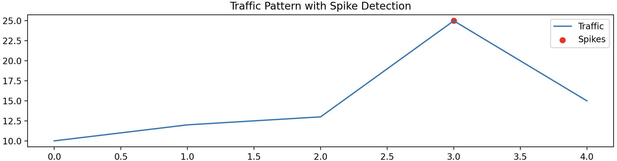
The most I love is workload_spike_detection in Traffic Pattern Detection problem, it is a simple problem to solve, but it is not easy to implement with Two-Pointer, and I think it is very important to understand the Two-Pointer and how to use it to solve the problem.
Workload spikes detected: False at: 15
Workload spikes detected: True at: 31
Workload spikes detected: False at: 12
Workload spikes detected: False at: 13
Using Two-Pointer to solve the problem, we can easily implement the workload_spike_detection function:
def detect_spike(self, value: float) -> bool:
    self.window.append(value)
    if len(self.window) < 2:
        return False

    prev_avg = sum(list(self.window)[:-1]) / (len(self.window) - 1)
    current = self.window[-1]
    # print(f"Prev avg: {prev_avg}, Current: {current}")
    print(f"Workload spikes detected: {(current - prev_avg) / prev_avg > self.threshold} at: {current}")

    return (current - prev_avg) / prev_avg > self.threshold
deque (Double-ended Queue) library is used to implement the sliding window, it is a double-ended queue, which means that it can be used to implement both FIFO (First-In-First-Out) and LIFO (Last-In-First-Out) operations.
So, Why Use Deque:
- O(1) operations at both ends
- Memory efficient with maxlen
- Thread-safe operations
- Built for sliding window patterns
- No reallocation needed
- Faster than list for window operations ```
3. Divide and Conquer
Pesudo code shows the scenario to use divide and conquer pattern:
def is_suitable_for_divide_and_conquer(problem):
    conditions = {
        "can_be_broken_down": True,      # Problem can be divided into smaller subproblems
        "overlapping_subproblems": False, # Subproblems are independent
        "recursive_pattern": True,        # Similar pattern at each level
        "combinable_results": True        # Results can be combined efficiently
    }
    return all(conditions.values())
- Critical for: Distributed data processing and parallel computing
- Practice with: Sorting problems (#23 Merge k Sorted Lists)
- Real application: MapReduce implementations, parallel data processing
In real world - data engineering case, we divided the data processing into small chunks to process it in parallel, and then combine the returns to get the final result. (Map-Reduce). On the other hand, we can split the process into multi pools to process the data in parallel. (Multiprocessing)
import multiprocessing
import numpy as np

def parallel_array_sum(array):
    def sum_chunk(chunk):
        return np.sum(chunk)

    # Number of cores
    num_cores = multiprocessing.cpu_count()

    # Split array into chunks
    chunks = np.array_split(array, num_cores)

    # Create pool of workers
    pool = multiprocessing.Pool(processes=num_cores)

    # Map the sum_chunk function to all chunks
    chunk_sums = pool.map(sum_chunk, chunks)

    # Close the pool
    pool.close()
    pool.join()

    # Combine results
    return sum(chunk_sums)

# Usage example
arr = np.array(range(1000000))
total_sum = parallel_array_sum(arr)
print(f"Sum: {total_sum}")
Tech3. Dynamic Programming
Dynamic Programming is a method for solving complex problems by breaking them down into simpler subproblems and solving each subproblem only once. It is particularly useful for optimization problems, where the goal is to find the best solution among a set of possible solutions.
Different wtih Divide and Conquer, Dynamic Programming is a method for solving complex problems by breaking them down into simpler subproblems and solving each subproblem only once. It is particularly useful for optimization problems, where the goal is to find the best solution among a set of possible solutions.
- Critical for: Resource optimization and caching strategies
- Practice with: Optimization problems (#322 Coin Change)
- Real application: Query optimization, resource allocation in data pipelines
For easier to understand the DP(Dynamic Programming), splitting file during partition is the good example of how data is splitted and optimial for reading operation. Using function below:
def calculate_num_files(data_size, partition_size):
    num_files = data_size // partition_size
    if data_size % partition_size > 0:
        num_files += 1
    return num_files
To get the number of fize of we have contraints and partition file size.
❯ python3 dynamic-programming-partition-strategy.py
Starting Dynamic partitioning strategy for File Partition
Data has partitioned with size is: 50
Number of partitioned files: 2
Size of each partitioned file: [50, 50]
Another example of DP with Data Quality Checks which I love one. I experienced with most of data quality project, I believe “Good data is bettern than Big data”. That means no matter how big data you put in platfrom; it is garbage if bad-quality.
def _run_validation(self, data_chunk, rules):
    """Run validation checks on data chunk using specified rules"""
    validation_results = {}
    for rule in rules:
        if rule == 'not_null':
            validation_results[rule] = data_chunk.notnull().all()
        elif rule == 'positive_values':
            validation_results[rule] = (data_chunk > 0).all()
        # Add more validation rules as needed
    return validation_results
Tech4. Greedy Method
“If you’re hungry at a buffet, taking the first good dish you see is greedy. It might no be the best strategy for whole meal and health, but it works for now.”
Greedy strategy is the “simple but work” solution and less latency for processing data. it is a good approach for real-time decision making in data pipelines.
class GreedyOptimizer:
    def schedule_tasks(self, tasks):
        tasks.sort(key=lambda x: x['cost'])

        current_time = 0
        scheduled_tasks = []
        for task in tasks:
            if current_time + task['duration'] <= task['deadline']:
                current_time += task['duration']
                scheduled_tasks.append(task)
        return scheduled_tasks

# Usage
tasks = [
    {'name': 'task1', 'duration': 2, 'deadline': 5},
    {'name': 'task2', 'duration': 3, 'deadline': 7},
    {'name': 'task3', 'duration': 4, 'deadline': 10},
    {'name': 'task5', 'duration': 9, 'deadline': 30},
    {'name': 'task4', 'duration': 5, 'deadline': 20}
]
optimizer = GreedyOptimizer()
scheduled_tasks = optimizer.schedule_tasks(tasks)
print(f"Scheduled tasks: {scheduled_tasks}")
The output will be:
Scheduled tasks: [
  {'name': 'task1', 'duration': 2, 'deadline': 5},
  {'name': 'task2', 'duration': 3, 'deadline': 7},
  {'name': 'task3', 'duration': 4, 'deadline': 10},
  {'name': 'task4', 'duration': 5, 'deadline': 20},
  {'name': 'task5', 'duration': 9, 'deadline': 30}
]
- Critical for: Real-time decision making in data pipelines
- Practice with: Scheduling problems (#1326 Minimum Number of Taps)
- Real application: Task scheduling, resource allocation
Tech5. Backtracking
For back to the track and find the best solution or feasible solution What is the Recursion?
The process in which a function calls itself directly or indirectly is called recursion and the corresponding function is called a recursive function.

How it works:
* Performing the same operations multiple times with different inputs.
* In every step, we try smaller inputs to make the problem smaller.
* A base condition is needed to stop the recursion otherwise infinite loop will occur.
Let’s think about What is different between Backtracking and Recursion ? . Basically, we add the Condition before call recursive function in backtracking.
def implement_backtracking():
    # 1. Define the state space
    state_space = define_state_space()

    # 2. Define constraints
    constraints = define_constraints()

    # 3. Implement validation
    def is_valid(state):
        return check_constraints(state, constraints)

    # 4. Implement backtracking logic
    def backtrack(state):
        if is_complete(state):
            return state

        for candidate in get_candidates(state):
            if is_valid(state + [candidate]):
                result = backtrack(state + [candidate])
                if result:
                    return result
        return None
Use for
- Critical for: Query optimization and dependency resolution
- Practice with: Combination problems (#39 Combination Sum)
- Real application: Query path optimization, workflow dependency resolution
def add_task(self, task_id, dependencies=None):
    self.tasks[task_id] = task_id
    self.dependencies[task_id] = dependencies or []

def resolve_execution_order(self):
    def backtrack(ordered_tasks, remaining_tasks):

pipeline = DataPipeline()
pipeline.add_task('extract_data')
pipeline.add_task('transform_data', ['extract_data'])
pipeline.add_task('load_data', ['transform_data'])
execution_order = pipeline.resolve_execution_order()
With result, we optimally order the tasks, which could be use in DAG organizer.
❯ python3 backtracking-piepline-organizer.py [‘extract_data’, ‘transform_data’, ‘load_data’]
Preparation Tips:
- Define clear constraints
- Implement efficient validation
- Handle edge cases
- Monitor performance
- Include logging and debugging
- Test with various scenarios
TODO: Check the Algo in hyperlink
I remember the [BackTracking] algorithm which is quite similar with theAutomotive Control Algo I learned when I was in university. The Right Side Following Algo is for automatic robot tracking. I combined that algorithm with PID Algo for controlling the speed to wheels.
I image the error recovery scenario when we are trying to resolve the problem, the causes of issue might be failure_points = ['database_crash', 'network_timeout', 'memory_overflow'] and we have several actions can perform to quickly recover system back recovery_actions = ['restart', 'retry', 'failover'].
Tech6. Breadth-First vs Depth-First
A long side with Vector data type, the Graph is the most complex and hard to handle but it quite benefit to visualize and store data has complex relationship.
Queue BFS vs Stack DFS
# BFS uses Queue (FIFO)
queue = deque([start_vertex])
current = queue.popleft()  # Remove from left (first in)

# DFS uses Stack (LIFO)
stack = [start_vertex]
current = stack.pop()  # Remove from right (last in)
- Critical for: Data lineage and dependency graph traversal
- Practice with: Graph problems (#207 Course Schedule)
- Real application: Data pipeline dependency resolution, schema validation
==> Finding out the 4 dependencies and 1 independent in a Graph.
In the example we will know 2 data structures: Queue and Stack and it right correctsponding the FIFO and FILO. We will figure out them later in below and in this part only know the mechanism of each data type; it basically is explained in the following.
Queue:  -> 1,2,3,4,5 ->
Deque:  5,4,3,2,1 #(First In - First Out)

Stack: --> 1,2,3,4,5 ]
UnStack: 1,2,3,4,5 ] #(First in - Last Out)
Tech7. Hash Tables for Lookup
In my whole time when I work in the industry as data engineer, data architect. I have seen many times that we use the Hashing algorithm to cutting edge the data processing and querying and storing data. It is a most important part in software engineering and data processing.
I lot of technical aplications that apply the hashing, in data management that we use hash-table to store the data, and in caching to store the frequently used data. It is very important to understand the hashing and how to use it to optimize the performance of data processing and querying.
Use it for:
- Critical for: Data deduplication and caching
- Practice with: Lookup problems (#1 Two Sum)
- Real application: Caching systems, data deduplication
With Python, A hash table is a data structure that implements an associative array abstract data type, a structure that can map keys to values using a hash function. But in data privacy management, we use the hash table to store the sensitive data, and we need to use the hash function to make the data privacy.
Masked Records:

Record:
id: 1
full_name: J*** D**
email: j******e@example.com
phone_number: ******7890
credit_card: XXXX-XXXX-XXXX-1111
ssn: XXX-XX-6789
address: 123 ********************
birth_date: XXXX-XX-XX (1990)
Always use the logging and rollback to functions to mask the sensitive data.
Processing History:
    {'20250108_213609':
        {'total_records': 2,
        'processed_at': datetime.datetime(2025, 1, 8, 21, 36, 9, 762007),
        'fields_masked': ['email', 'phone_number', 'credit_card', 'ssn', 'full_name', 'address', 'birth_date']
        }
    }
It helps to monitor the process of maksing data. The practice to make the data privite is using batch processing and write Dynamic Programing to process the xx chunk of data and mask the yy fields (attributes) in the data.
masked_records = handler.process_batch(records, sensitive_fields)
Tech8. Binary Search Pattern
Binary Search is a divide-and-conquer algorithm that finds the position of a target value within a sorted array by repeatedly dividing the search interval in half.
Use it for:
- Critical for: Log analysis and time-series data querying
- Practice with: Search problems (#33 Search in Rotated Sorted Array)
- Real application: Log parsing, time-series data analysis
self.index_map = {}  # Hash table for quick timestamp lookup
self.value_heap = []  # Heap for maintaining sorted values
You might use the Search Function a lot when doing the data profiling and analysis, with SQL query there is a like operator to the find the value in the string. And if you want to find the value in the array, you can use the in operator. If you have a Data Governance tool like OpenMetadata, you can easily find the lineage and data catalog by searching the technical and business term.
With advantage of Graph with super complex relationship a long with Graph Algorithms, finding the vertex of edge is much more easier. I have pubpished the Generating Data Lineage with Graph in my blog post, the project provides a solution for generating and visualizing data lineage based on table DDLs and ETL job metadata. The solution includes a Python script for generating data lineage information and a React application for visualizing the data lineage as a Directed Acyclic Graph (DAG).
The most stack for searching and logging analysis is the ELK Stack and it is a great tool for data engineering. It is a combination of Elasticsearch, Logstash, and Kibana. Elasticsearch is used for storing and indexing the data, Logstash is used for processing and transforming the data, and Kibana is used for visualizing and analyzing the data. The ELK Stack is widely used in the industry for its scalability, reliability, and ease of use. Try it out with the Toidicodedao did a very good tutorial for demonstrating the ELK. It follows what I have mentioned in the 5 layer of every data pipeline.
Or you can find the Draw.io design file in the store
Tech9. Stack-based Problems
- Critical for: Expression parsing and workflow management
- Practice with: Parentheses problems (#20 Valid Parentheses)
- Real application: ETL workflow management, query parsing
Preparation Tips:
- Focus on problems tagged as Medium difficulty on LeetCode
- Practice implementations in Python (most common in data engineering)
- Time yourself to simulate interview conditions
- Review real system design questions from companies
Remember: While these patterns may seem academic, they form the foundation of efficient data processing systems. Regular practice not only prepares you for interviews but improves your ability to design scalable data solutions.
_ TO BE CONTINUED …_